What is an ESOP (Employee Stock Ownership Plan)?
An ESOP is an employee benefit that provides the company’s workers the opportunity to participate in having an ownership interest in the firm.
As participating employees become shareholders, they have an interest in seeing the company’s stock perform well and are encouraged to do what’s best for shareholders.
Thus, ESOPs serve to align the interest of the employees and company owners.
ESOPs can take many forms:
- Issuance of company shares to employees such that they become a shareholder immediately (immediate vesting), or
- more commonly, Granting Stock Options such that the employee has the right to become a shareholder at some point in the future subject to the fulfilment of certain conditions (known as vesting conditions).
What are the vesting conditions?
1. Service Condition
The employee has to work in the company for a specified period of time before being able to exercise their Options.
Example 1– a company grants 1000 Options to an employee which vests after 3 years (the vesting period). In this case, the employee has to work in the company for 3 years (after being granted the Options) and then only can they exercise the Options. Should the employee leave during the vesting period, the Options are forfeited.
Example 2 – a company grants 1000 Options to an employee which vests over 4 years as follows:
- 25% vest one-year after grant date,
- 25% vest two-years after grant date,
- 25% vest three-years after grant date, and
- the remaining 25% vest four-years after grant date.
In this case, the employee has to work in the company for:
- 1 year after being granted the Options and then can exercise 250 Options;
- 2 years and then can exercise a further 250 Options;
- 3 years and then can exercise a further 250 Options; and
- 4 years and then can exercise remaining 250 Options.
Hence there are 4 vesting periods in this example.
2. Performance Condition
The employees can exercise their Options if the company can achieve (i) prescribed Revenue or Profit targets within a specified time-frame or (ii) specified increase in the share price.
Accounting for Share Options
Let’s use start-ups as an example. As they are strapped for cash, most start-ups issue Shares or Share Options to attract, incentivise and retain talented employees.
While there is no actual cash outflow when a company issues Shares or Share Options to Employees, the accounting standard requires the company to recognize and measure these transactions in accordance with IFRS 2- Share-based Payment (US GAAP- ASC 718 – Stock Compensation).
This article will focus on the valuation of equity-settled share-based payment transactions i.e., where the company receives services (from employees) as consideration for equity instruments (shares / share options).
Recognition
IFRS 2 share-based payment transaction is only recognized when the services received (from employees) are actually performed.
The services received (from employees) should be recognized as expenses (debit) in the income statement. The credit side is recognized in equity.
Dr Employee Benefits
Cr Shares (Note 1) / Share Options (Note 2)
Note 1
The issuance of Shares can be issued as fully vested, i.e., an Apple employee can receive 100 AAPL shares (no conditions attached)
If this is the case, the issuance is presumed to relate to past service (by the employee), requiring the full amount of the fair value of the AAPL Shares on Grant Date to be expensed immediately.
Shares with Vesting Conditions
The issuance of Shares can also be issued with Vesting Conditions, e.g., a Microsoft employee can receive 100 MSFT shares only after working 3 years in the Company.
In this example, the issuance of Shares to the employee is with a three-year vesting period and is considered to relate to services over the vesting period. Therefore, the fair value of the MSFT Shares determined at the Grant Date, should be expensed over the vesting period (i.e., after each year of service).
Note 2
The issuance of Share Options can be issued as fully vested but, in most cases, Share Options are issued with Vesting Conditions, for example, a 3-year vesting period where 100% of the Share Options vest after the employee works for 3-years in the Company (thereafter the employee can exercise their Options).
However, since the Share Options relate to services over the vesting period, for accounting purposes, the fair value of the Share Options (determined at the grant date), should be expensed equally over the vesting period (i.e., after each year of service)..
Measurement
As the value of services received from employees cannot be reliably measured, IFRS 2 states that the entity should measure the value by reference to the fair value of the Share Options granted at the Grant Date.
The Fair Value of the Share Options is determined only at Grant Date, regardless of the term of the Options or the length of the vesting period.
When determining the Fair Value of the Share Options, only Market Conditions (share price and volatility), should be taken into account. Non-market conditions, such as service conditions and performance conditions should be adjusted in the number of Share Options expected to vest each year.
Refer to the example below:
Company XYZ grants a total of 100 share options to 10 members of its executive management team (10 options each) on 1 January 20X5. These options vest at the end of a three-year period. The company has determined that each option has a fair value at Grant Date equal to $15 per Option.
1 January 20X5
There are no Share-based transactions recognized at Grant Date as no services have yet been performed (by the executive management team)
31 December 20X5
As at 31 Dec 20X5, 1 year of services have been received out of the 3 years vesting period, therefore the Company should expense 33.3% (1 / 3).
Furthermore, as all 10 Executives are still employed, the Company expects that all 100 options will vest.
Dr Share-based payment expense $500
Cr Equity: Share Options $500
(10 Executives x 10 Options x $15/option) * 1/3 years
31 December 20X6
As at 31 Dec 20X6, 2 years of services have been received out of the 3 years vesting period, therefore the Company should have expensed 66.7% (2 / 3). Bear in mind 33.3% was already expensed in 20X5, therefore the Company should only expense a further 33.3% in 20X6.
Furthermore, while all 10 Executives are still employed, the Company now expects that 1 will leave during the vesting period and 90 options will vest.
Dr Share-based payment expense $400
Cr Equity: Share Options $400
[(9 Executives x 10 Options x $15/option) * 2/3years ] less $500 (from year 1 expense)
31 December 20X7
As at 31 Dec 20X7, 3 years of services have been received out of the 3 years vesting period, therefore the Company should have expensed 100%. Bear in mind 66.7% was already expensed up to 20X6 therefore the Company should only expense the remaining 33.3% in 20X7.
Furthermore, only 8 Executives are still employed, therefore 2 Executives have forfeited their 20 Options and a total of 80 Options vested at the end of year 3.
Dr Share-based payment expense $300
Cr Equity: Share Options $300
[(80 Options x $15/option) * 3/3 years] less ($500 + $400) (year 1 and year 2 expenses)
Modifications, cancellations, and settlements
The determination of whether a change in terms and conditions has an effect on the amount recognised depends on whether the fair value of the new instruments is greater than the fair value of the original instruments (both determined at the modification date).
Modification of the terms on which equity instruments were granted may have an effect on the expense that will be recorded. IFRS 2 clarifies that the guidance on modifications also applies to instruments modified after their vesting date. If the fair value of the new instruments is more than the fair value of the old instruments (e.g. by reduction of the exercise price or issuance of additional instruments), the incremental amount is recognised over the remaining vesting period in a manner similar to the original amount. If the modification occurs after the vesting period, the incremental amount is recognised immediately. If the fair value of the new instruments is less than the fair value of the old instruments, the original fair value of the equity instruments granted should be expensed as if the modification never occurred.
The cancellation or settlement of equity instruments is accounted for as an acceleration of the vesting period and therefore any amount unrecognised that would otherwise have been charged should be recognised immediately.
New equity instruments granted may be identified as a replacement of cancelled equity instruments. In those cases, the replacement equity instruments are accounted for as a modification. The fair value of the replacement equity instruments is determined at grant date, while the fair value of the cancelled instruments is determined at the date of cancellation, less any cash payments on cancellation that is accounted for as a deduction from equity.
How to determine the Fair Value of the Options at Grant Date?
First, we have to answer what is fair value? Fair value is the price transacted between market participants in an orderly transaction on a certain date.
In most cases, fair value can be referenced to the market price (e.g., the last traded price of a stock on the stock exchange)
However, in some cases, when there is no active market, fair value can be determined using valuation techniques.
Since Share Options issued to employees are not traded on any active market, their fair value is determined using Option Pricing Models.
Options Overview
Definitions
- An Option is a financial instrument that derives its value from an underlying security such as a stock.
- An Option contract offers the holder the opportunity to buy (or sell) the underlying security (hereafter referred to as Stock).
- The benefit of holding an Option is that the holder is not required to buy (or sell) if they choose not to. The Option will simply lapse if it is not exercised.
There are 2 types of Options:
Exercise Price / Strike Price (“X”) – the specified price in the Option contract at which the holder is entitled to buy (call) or sell (put) the underlying stock.
Spot Price (S) – the current market price of the stock.
1. Call Options – give the holder the right, but not the obligation, to buy the stock at a specified price within a specific time period. A call buyer profits when the stock price increases.
When S > X, the Call Option is profitable (“in the money”) and the buyer will exercise.
2. Put Options – give the holder the right, but not the obligation, to sell the stock at a specified price within a specific time period. A short seller profits when the stock price decreases.
When X > S, the Put Option is profitable (“in the money”) and the seller will exercise.
American vs. European Options
American Options – owners of American Options can exercise any time before the Options expire.
European Options – owners of European Options can exercise only on expiration date (i.e., at the end of the Options life).
Option Pricing Models
There are 3 Option Pricing Models
- Black-Scholes Merton Model;
- Binomial Model; and
- Monte-Carlo Simulation Model
This article serves to give you an overview of the different models. You do not need to get too hung up on understanding the mathematics & technicalities of each model. More importantly from a practical stand point, you need to understand:
- how to use the model,
- what are the model inputs, and
- how each input affects the Option value.
This will be covered in later articles.
Black-Scholes Merton Model
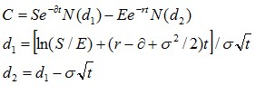
The Black Scholes model (BSM) is a commonly used mathematical model for pricing an Option. The model estimates the variation over time of the underlying stock, and derives the price of the Option using the implied volatility of the underlying stock.
The standard BSM model can only be used to value European options, an Option that can only be exercised on expiration date, (i.e., at the end of the Option life)
Binomial Option Pricing Model
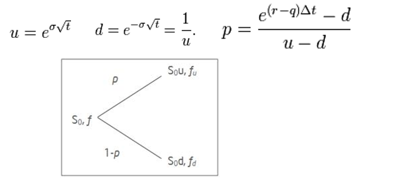
The binomial option pricing model (Binomial Model) uses an iterative procedure, allowing for the specification of nodes, or points in time, during the time span between the valuation date and the option’s expiration date.
Therefore, unlike the standard BSM model, the Binomial Model can be used to value American Options, an Option that can be exercised any time before its expiration.
Monte-Carol Simulation Model
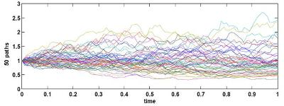
Monte Carlo simulations are done using computer software to model the probability of different outcomes and therefore can be used to value an option with multiple sources of uncertainty.
A Practical Application of the Black-Scholes Merton Model
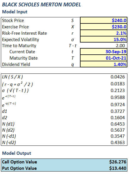
Now I will walk you through the Black-Scholes Model using the following example:
Assume today is 30 September 2019.
Jeff holds 600,000 Call Options which gives him the right to acquire 600,000 Apple Shares two years later, on 1 October 2021 (i.e., on expiration date of the Call Options) at a strike price of $230/share.
Determine the valuation of Jeff’s Options today (30 September 2019)?
Step 1 – Determine if the Black Scholes Model is appropriate for your Valuation
Jeff’s Options are European Options as they vest (i.e., can only be exercised) at the end of the Options life.
Black Scholes Model is an appropriate model for valuing European Options (not American Options).
Step 2 – Determine your Valuation Date
The Options will be valued as of today, 30 September 2019 (the “Valuation Date”).
Step 3 – Identify each input to the BSM Model
Stock Price (indicated by the symbol “S”)
Should be the market price of Apple shares on Valuation Date (i.e., 30 September 2019).
S = $240
Exercise Price (indicated by the symbol “X”)
Should be the price per share at which Jeff is entitled to buy/strike Apple shares in the future.
X = $230
Risk-free Interest Rate (indicated by the symbol “r”)
The risk-free rate is the interest rate on a government bond.
r = 2.1%
Volatility (indicated by the symbol “σ”)
Should be the degree of variation/fluctuation of Apple’s share price which is expected over the next 2-years (i.e., over the life of the Options).
σ = 15%
Time to Maturity (indicated by the symbols “T – t”)
The remaining life of the Options (i.e., the period of time from Valuation Date (t) up to Maturity/Expiration Date (T)
t – 30/9/2019
T – 1/10/2021
T – t = 2.0 (year)
Dividend Yield (indicated by the symbol “q”)
Should be the dividend yield expected from Apple shares over the next 2-years (i.e., over the life of the Options).
q = 1.4%
Step 4- Analyse the Result and Perform Sensitivity Analysis (if necessary)
The Value per Call Option on 30 September 2019 is $26.276 per Option.
The total value of Jeff’s 600,000 call options is about $15.77 million.
A Practical Application of the Binomial Model
Now I will walk you through the Binomial Model using the following example:
Company XYZ has granted share options to its employees on 3 January 20X5 (the “Grant Date” or “Valuation Date”).
Company XYZ produces and sells processed fruit products in China and internationally. It is listed on the stock exchange of Hong Kong.
Key Terms of the Options
6 million Options were granted in total
50% of the Options will vest on 31 December 20X5 (“Vest Date 1”)
25% of the Options will vest on 31 December 20×6 (“Vest Date 2”)
25% of the Options will vest on 31 December 20×7 (“Vest Date 3”)
The Options mature on 31 December 20×8 (the “Expiration Date”)
Exercise Price of the Options is HKD 1.70
Please calculate the fair value of the Options at Grant Date in accordance with IFRS 2 – Share-based payments.
Step 1 – Determine the Valuation Methodology
The Options granted by XYZ Ltd are American Options as there is possibility of early exercise of the Options before its expiry date.
The Binomial Option Pricing Model is an acceptable model which is commonly used by valuation practitioners in valuing (American style) employee share options.
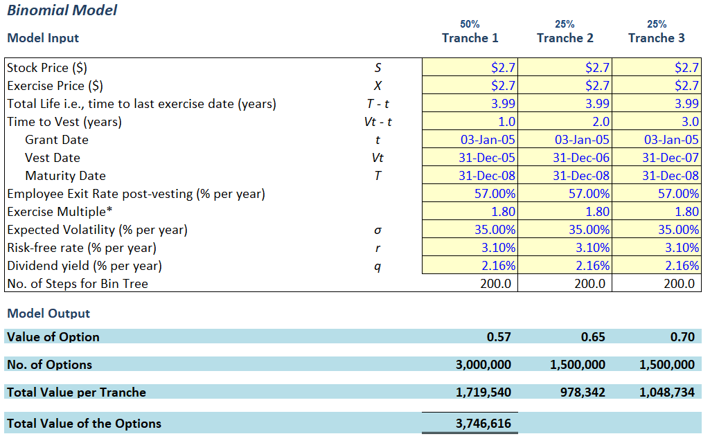
As there are 3 tranches (because there are 3 vesting dates), we will need to set up 3 binominal models (1 for each Tranche)
Step 2 – Determine the inputs to the Binomial Model
Spot Price – (indicated by the symbol “S”)
This will be XYZ Ltd’s share price on Valuation Date (i.e., 3 January 20X5) which can be obtained from the Hong Kong Exchange.
Spot Price is HKD 2.70
In this example, since XYZ Ltd is a publicly listed company, obtaining the Spot Price is relatively easy. If XYZ Ltd was a private company, the Spot Price would need to be determined using certain valuation techniques.
Exercise Price -(indicated by the symbol “X”)
This is the price per share at which Option holders are entitled to buy/strike XYZ shares in the future which is stated on the Options Grant Letter issued to employees.
In this case the Exercise Price is HKD 2.70 as stated in the Grant Letter
Kindly note that the Options are “at-the-money”. If S > X (i.e., if the Exercise Price was lower than HKD 2.70), than the Options are “in-the-money”. If S < X (i.e., if the Exercise Price was higher than HKD 2.70) than the Options would be “out-of-money”.
Time to Maturity- (indicated by the symbols “T – t”)
This is the remaining life of the Options i.e., the period of time from Valuation Date (t) up to Maturity/Expiration Date (T)
t – 3/1/20X5
T – 31/12/20X8
T – t = 4.0 (years)
Time to Vest- (indicated by the symbols “Vt – t”)
This is the time it takes for the Options to become exercisable i.e. the period of time from Valuation Date (t) up to when the Options vest (Vt)
t – 3/1/20X5
Vt 1 – 31/12/20X5, Vt 2 – 31/12/20X6, Vt 3 – 31/12/20X7
Vt 1 – t = 1.0 (years), Vt 2 – t = 2.0 (years), Vt 3 – t = 3.0 (years)
Employee Exit Rate Post-Vesting (% per year) –
This is the annual staff turnover rate (“churn”) expected over the life of the Options.
To determine the expected staff turnover rate, we can make reference to XYZ Ltd’s past 3-years historical staff turnover rate as a predictor for its future staff turnover rate.
The appropriate way to calculate the historical staff turnover rate would be to divide the number of staff who were still employed at the company at the beginning of the year but left during the year by the total number of staff employed at the beginning of the year (refer below).
We obtained employee data from XYZ Ltd and performed the following analysis:
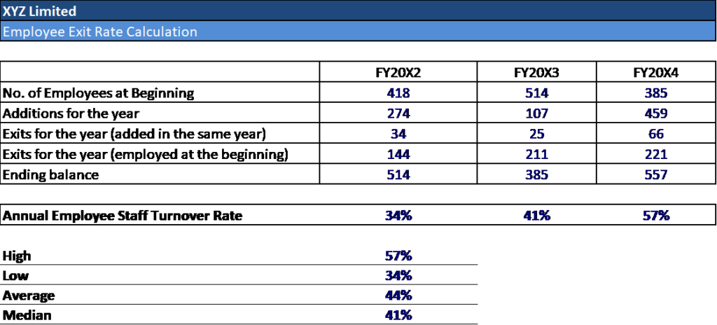
Typically, using the Average of the past 3-years historical data to extrapolate the future expected Staff turnover rate would be acceptable. However, in this example, there is a blatant upward trend identified in the Staff turnover rate.
Therefore, it would make more sense to adopt the High Exit rate of 57% (which is the staff turnover rate for 20X4) in our model. Due to the upward trend, the expected exit rate could be higher than 57%. As such, it is recommended to perform sensitivity analysis on Exit rate assumption using higher rates, say, 60%, 65% and 70%.
The higher the Post-vesting Exit Rate, the lower the Option Value
Exercise Multiple –
The exercise multiple factors in early exercise behavior (i.e. assuming the grantees would exercise the Options when XYZ’s stock price equals a certain multiple of the Option’s exercise price).
For example, an Exercise Multiple of 2x assumes that the Grantees would exercise the Options when XYZ’s Share Price is 2x its Exercise Price.
There are 2 ways to determine the Exercise Multiple.
- Historical Employee Exercise Data – make reference to historical exercise multiples based on previous exercise behavior of XYZ’s employees.
- If such data is not available or if no employee share options for XYZ have been exercised in the past, then the exercise multiple is based on empirical studies.
Overseas empirical research (e.g. Carpenter 1998, Huddart and Lang 1996, Mun 2004, etc) shows that a typical early exercise multiple ranges from around 1.5× to 3.0× (i.e. employees typically exercise their share options when the stock price is around 1.5× to 3.0× of the exercise prices) and that option holders in more senior management positions may require higher exercise multiples.
If the Options were granted to Directors of XYZ Ltd, then we would adopt an Exercise Multiple which is on the high-end of the 1.5x to 3.0x empirical research range, say 3.0x.
However, in this case, since the Options were issued to low and mid-level employees of XYZ Ltd, we adopt an Exercise Multiple which is on the lower-end of the 1.5x to 3.0x empirical research range, say 1.8x.
Expected Volatility – (indicated by the symbol “σ”)
The volatility factors in the degree of variation/fluctuation of XYZ Ltd’s share price which is expected over the life of the Options.
Valuation practitioners typically make reference to historical volatilities when determining future expected volatility.
In this example, we consider XYZ Ltd’s shares own historical volatility to be representative of its future volatility.
The period of historical volatility assessed should match the Options term (i.e., the life of the Options). Since the term of Options granted by XYZ Ltd is 4.0 years, we will make reference to the historical 4-year volatility of XYZ Ltd‘s share.
Based on our calculation, the historical 4-year volatility of XYZ Ltd is 35%
Kindly note, the higher the expected volatility, the higher the Options Value (and visa versa). This is because, the more up and down movements a share price has, the greater the chances of it going above the Exercise Price and therefore becoming “in the money”. “In-the-money” Options are more valuable.
Please refer here for all you need to know when determining expected volatility.
Risk-free rate – (indicated by the symbol “r”)
The risk-free rate typically used in the Binomial Model is the interest rate on a government bond as of the Grant Date.
Which country’s government bond should we make reference to?
The country of the government issuing the bond (including the bond’s currency) should match the currency of the Exercise Price. In XYZ’s example, since the Exercise Price of the Options is HK$, we make reference to a Hong Kong Government Bond.
The term of the Government bond should match the term of the Options. In our example time to maturity is 4 years. However, the Hong Kong Government does not issue 4-year bonds, therefore we interpolate and make reference to the mid-point of a 3-year and 5-year government bond.
The 4-year interpolated yield on a HK government bond as of Grant Date sourced from Bloomberg is 3.1%.
Dividend Yield – (indicated by the symbol “q”)
The Option holder does NOT receive dividends from the underlying stock. Therefore, the higher the dividend yield on the stock, the lower the value of Options. This is to capture the fact that by holding an Option instead of the actual stock, the Option holder is missing out on these dividends.
Since we are concerned with the dividend yield expected over the life of the Options, we ask Management of XYZ Ltd to confirm their future dividend policy (i.e., do they expect to maintain the same payout ratio or maintain the same dividend per share over the next 4 years).
Management confirm that future dividends will be similar to historical. As a result we analyse XYZ Ltd’s last 3 year dividend yields as follows:
Kindly note we calculate dividend yield as follows:
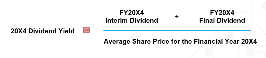
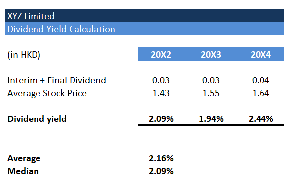
Based on the above, we adopt an expected dividend yield of 2.16% in the Binomial model.
Step 4- Analyse the Result and Perform Sensitivity Analysis (if necessary)
The Value per Call Option depends on which Tranche.
- Tranche 1 – HKD 0.57 per Option
- Tranche 2 – HKD 0.65 per Option
- Tranche 3 – HKD 0.70 per Options
(Notice the longer the time to vest, the higher the Option Value. This is because, when an Option has more time to vest, there is a greater chance of the Option becoming “in-the-money”)
The total fair value of Options issued by XYZ Limited is about HK$ 3.75 million.