
The discounted cash flow (DCF) model is probably the most versatile technique in the world of valuation. It can be used to value almost anything, from business value to real estate and financial instruments etc., as long as you know what the expected future cash flows are.
This article is going to focus on the most common application of a DCF, which is valuing a business. We will explain the concept behind and give you a step by step walkthrough on how to set up your spreadsheet and formulas to calculate the value of a business.
Before we start, you need to have the following in order to do a basic DCF:
- A forecast that includes at least the P&L;
- Financial statements as of or close to your valuation date (see below); and
- Microsoft excel or equivalent spreadsheet tools.
Valuation Date
Due to the time value of money, $1,000 today is worth more than $1,000 next year.
Also, the DCF approach values a business at a single point in time (i.e., the Valuation Date). So the very first step is to determine the Valuation Date of your DCF.
Next you need to determine the Expected future cashflows from the Valuation Date onwards (since the DCF only incorporates future cash flows into the valuation).
In our example, we set the Valuation Date to be 31 December 2018.
Projection Period and Terminal Year
Businesses are assumed to be a going concern (i.e., they operate into the foreseeable future). As we mentioned above, the DCF incorporates expected future cashflows into the valuation for the foreseeable future. These expectations are built into the DCF as follows:
1. The Projection Period
The projection period refers to the time period that your forecast covers. Valuation best practice recommends the projection period to extend until the business has matured and growth stabilized.
For example, start-up businesses have high growth expectations and should incorporate a longer projection period as compared to a mature business. That being said, since we cannot predict the future, most forecasts typically go up to 3-years or 5-years. Some businesses may be able to forecast more accurately for even longer periods (say 10 years) because they have more predictable cashflows which could be due to signed agreements/concessions.
Ideally, you should set the projection period based on (i) the stage of the business and (ii) until the business has matured and stabilized. However you don’t want a projection period that’s too long (> 5 years) unless you have are confident on the expectations beyond this period.
2. The Terminal Year
So you are probably thinking, if my Projection Period is only 5 years, how do I incorporate future cash flows (for the foreseeable future) into my DCF ?
The answer is the terminal year!
The terminal year assumes that a business will continue to generate cash flows at a constant stable rate forever. That is why we stress the importance of the business having matured and stabilized during the projection period.
The terminal value is calculated in the terminal year and we will discuss more on how to do terminal value calculation later in this article.
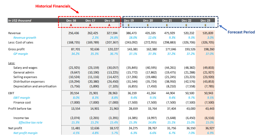
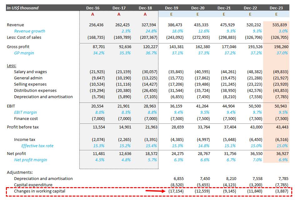
In our example, the projection period is from FY2019 to FY2023, with 2023 being the terminal year. Kindly note the Historical Financials are for reference only.
Converting Accounting Earnings into Cashflows
As indicated by its name, a DCF concerns only cashflows but not profits. Accounting profits could be very different from the cashflow due to accruals, receivables, capitalized investments etc. Consider a very simple example here: you sell a car for $100k, but the customer will pay you one year later. So your accounting profit for this year would be $100k (assuming $0 cost for simplicity), but your cash flow would be $0. So bear in mind, in the world of valuation, only cash flow matters. Therefore what we need to do next is to convert our projected profits into projected cash flows.
Generally speaking, there are three adjustments required to convert accounting profit into cashflow.
Step 1:
Add back the depreciation and amortization charges. Although they are considered expenses from an accounting perspective (thus deducted in the net profit), theses are non-cash items as there is no actual cashflow involved.
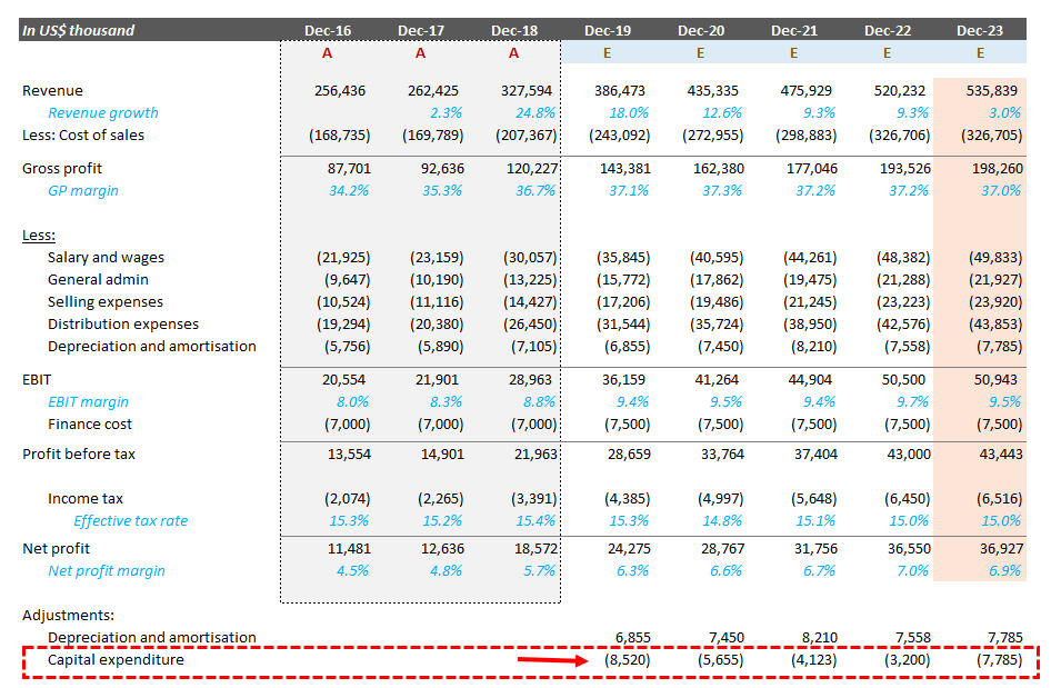
Consider this: MakDonald, a local restaurant bought a refrigerator two years ago for $1000 and the useful life of the refrigerator is 5 years. So every year, there will be a depreciation expense of $200. However, this $200 expense is not a cash flow because MakDonald has already paid the price of $1000 at the beginning (that payment was the cashflow). This is why we need to add back the depreciation and amortization charges.
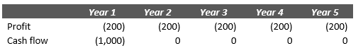
To adjust for the D&A expense, we simply add a line equal to the D&A expense in the Adjustments section as shown below:
Step 2:
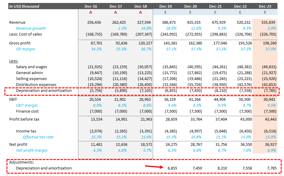
Deduct capital expenditure and investments. This is basically the reverse of step 1 above. Using the MadDonald case again, the $1000 cash outflow for buying the refrigerator is not counted as expense in the year in which it was paid because the $1000 was capitalized as a fixed asset on the balance sheet. Thus we need to deduct cash paid for these “investing activities” when calculating the cash flow for the year. Capital expenditure should also be projected when you prepare a forecast of the business (In our example it is provided ).
Step 3:
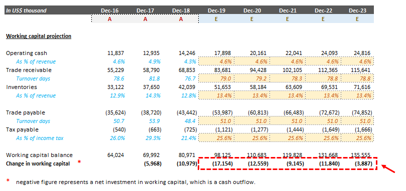
Changes in working capital. Working capital refers to the assets and liabilities that you need in running the business other than the fixed assets (which are subject to depreciation/amortization), some common items are operating cash, account receivables and payables etc. Very often, when your business is growing, you will need more inventory and operating cash. Furthermore your receivables will also be bigger due to more sales. Cash flow is required to finance the increase of working capital (and vice versa, cash will be released when working capital decreases). As cash flow is not captured in the income statement, we will need to adjust for these items in the DCF as well.
To determine the changes in working capital in the projection period, very often we will need to do a forecast by ourselves if we don’t have a projected balance sheet. Common techniques in forecasting the working capital includes benchmarking to the revenue and turnover days etc. For the sake of time we are not going to cover how to define working capital and forecasting method in this article. If you are interested to learn more, you may refer to our article here. In the sample forecast, we have already projected the working capital balance for you.
After adjusting the three items above, you have now successfully converted the profits into cash flows. But wait, which kind of cash flow are we talking about?
FCFF vs FCFE
There are two kinds of cash flows when it comes to DCF, one is free cash flow to firm (FCFF) and the other is free cash flow to equity (FCFE). Given the importance of this concept in DCF, we will explain a bit more what is FCFF and FCFE and how do they differ from each other.
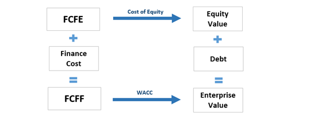
A company needs capital to run, and capital comes from either the Shareholders (Equity) or Debt holder (borrowings). So when a business generates cash flows, some of the cash flow will need to be paid to the debt holder first (in terms of financing cost, interest expenses) before the shareholders can receive any. Simply put, FCFF is the cash flow generated by the business as a whole (owing to both shareholders and debtholders) while FCFE is the cash flow entitled to shareholders only (i.e., debt holders have already been paid) .
The result from a DCF using FCFF will be enterprise value (the value of the business operation) while the result from FCFE will be the equity value (shareholder’s share of the company). Calculating FCFE would require you to project the financing cash flow (like borrowings, repayment and interest).
As the risk of equity and debt is different (i.e., lower risk to debt holder given more protection), FCFF and FCFE also require different discount rates in the DCF. FCFF is often discounted by weighted average cost of capital (WACC), while FCFE is discounted by cost of equity.
Both FCFF and FCFE are used when doing a DCF. Personally, I prefer using FCFF (except for certain industries, such as financial services) as it doesn’t require projecting the financing cash flows. So in this guide, we are going to do the DCF with FCFF.
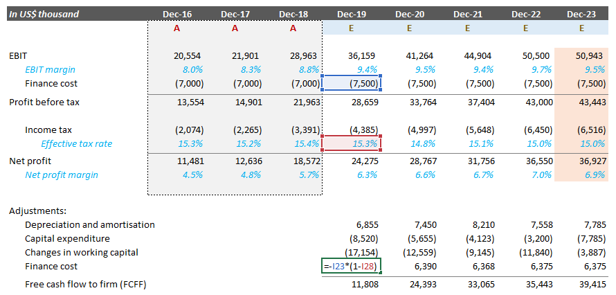
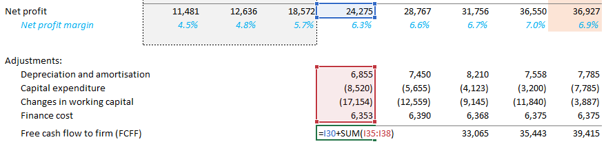
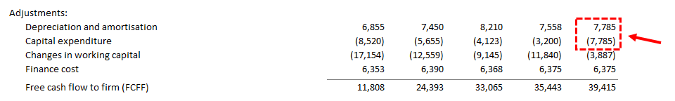
Given net profit has already deducted finance cost, to compute the FCFF, we need to add back the finance cost as illustrated below. Please note that we need to multiply the finance cost by (1 – tax rate) to account for the tax shield from the finance cost.
Terminal year normalization
So far we have considered cash flows in the forecast period. However, we would expect the business to run perpetually in general. So we need to take into account the cash flows beyond the terminal year as well.
There are a lot of ways to compute a terminal value. Common methods include Gordon growth model, H-model, exit multiples etc. We will discuss how to use the Gordon growth and H model in detail in later sections. For now, you need to know that these methods assume the business will enter a stabilized stage after the terminal year and will simply grow at a terminal growth rate (usually make reference to inflation rates, long term GDP growth rates etc.).
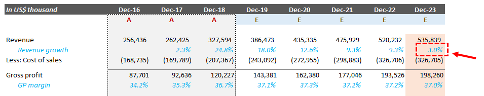
In the sample provided, you may notice the revenue growth is much lower and may look a bit artificial.
This is because we have normalized (stabilized) the terminal year projection. So why do we need to do a normalization? Think about this, when a business is growing at double digits, usually they are pouring a lot more resources to support the growth. For instance, you need to invest in production capacity (more capital expenditure), you will have more inventories and receivables (more investment in working capital).
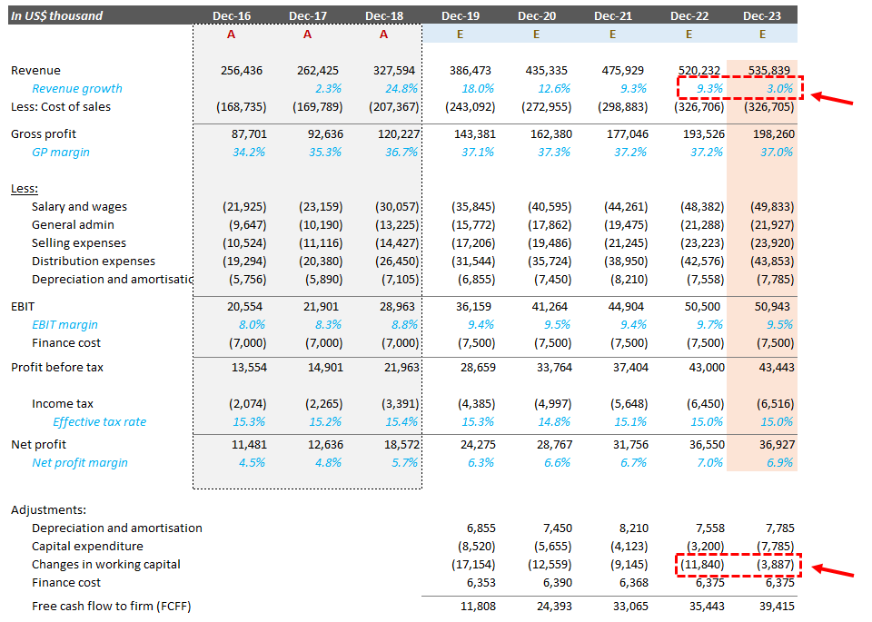
However, high growth can’t go on forever. If we calculate terminal value based on a year of high growth, we are assuming the level of capital expenditure and working capital investment required to support the high growth will also remain at the same level perpetually, which is definitely not the case when the growth rate drops to 3% (at 9.3% growth, changes in working capital is $11.8k. however, at 3% growth, it is just $3.8k).
Let’s have a look on how to do a normalization exactly.
Step 1:
Extend one year of the projection period, in this case, we have added the year 2023 to be our terminal year.
Step 2:
Using the terminal growth rate as revenue growth for the year (3% in this case)
Step 3:
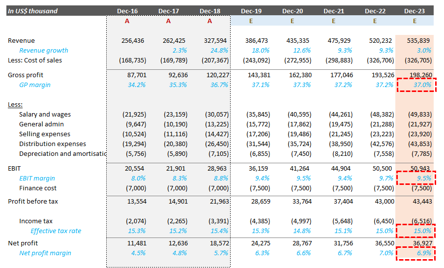
Estimate a long term GP margin, EBTI margin, tax rate and net margin. In our example, we reference to historical margins. We assume GP margin will stabilize at 37%, EBIT margin at 9.5%, net margin at 6.9% and effective tax rate at 15%.
Step 4:
Construct the cash flow with these terminal year assumptions
Step 5:
Calculate the changes in working capital, add back D&A expense and finance cost as usual.
Step 6:
For terminal year capital expenditure, please note it should always be slightly higher or at least equal to the Depreciation (D&A) expense. If fixed assets depreciate faster then your capital expenditure, then in the long-term, there will be no fixed assets left in the business which doesn’t make sense for a going concern. Most valuation specialists, normalize terminal year capital expenditure by making equal to D&A.
Discount the cash flows
Finally, we have the cash flows ready and we can do the discounting! Surprisingly, this is actually the most straight forward part in the DCF computation.
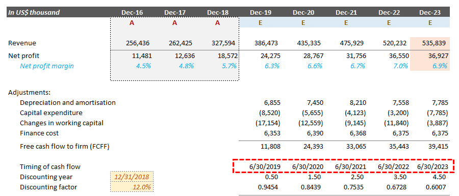
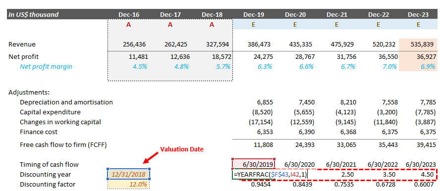
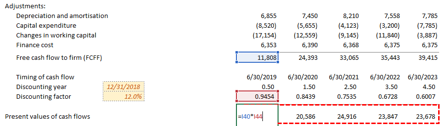
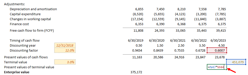
First step is to calculate how long should we discount. Back in school, we learnt that to calculate the present value of a cash inflow at 31 Dec 2019 on 31 Dec 2018, we need to discount such cash flow by 1 year. This is very true, but in the business world, you have cash flowing in and out all year around. It is not realistic to assume all cash come in at the end of the year. As such, generally we would assume the midpoint of the year (in this case 30 June 2019) as the time of cash flows to approximate cash flows coming in every month in the year. So the timing of cash flow for each of the year would be set at the middle of each year as follows:
Based on the timing of cash flows, we can calculate how long (in terms of year) they are from the valuation date. For the FY19 cash flow, we need to discount 0.5 year; For the FY20 cash flow, we need 1.5 year and so on.
Then we will compute the discounting factor, which basically follow the formula below:
Present value of cash flow = Cash flow / (1 + discount rate) ^ discounting period
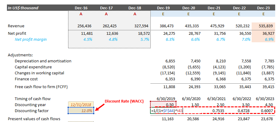
Getting the discount rate (WACC in this case) is another topic of its own and we generally estimate the WACC of a business using the CAPM model with reference to market data of listed comparable companies. You may refer to here for the tutorial on computing the discount rate.
After computing the discount factor, we can simply multiple it with the cash flow for the year to get the present values of cash flows.
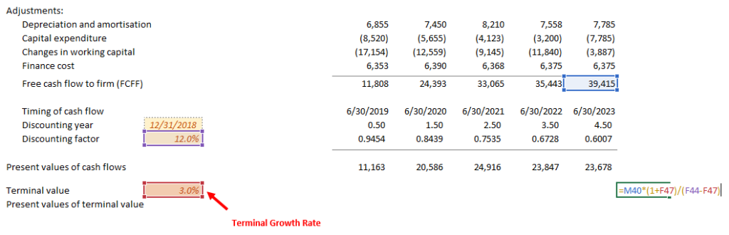
Terminal Value
Terminal value is the value of a business or project beyond the forecast period. Terminal value assumes a business will grow at a set growth rate forever after the forecast period. Terminal value often comprises a large percentage of the total assessed value. As mentioned earlier, there are many methods in computing the terminal value, here we will introduce Three of them, the Gordon Growth model, the H-model and the exit multiple method.
Gordon Growth Model
The Gordon Growth Model is used to determine the intrinsic value of a business based on a future series of cash flows that grow at a constant rate. It is a popular and straightforward variant of the dividend discount model (DDM). Basically it is equivalent to discounting below’s cash flow pattern to present.
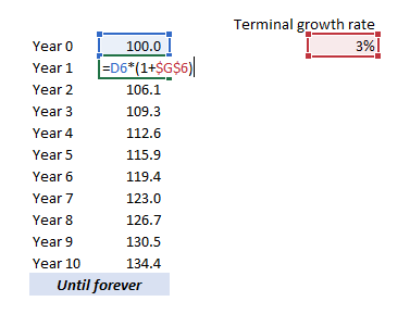
If we assume terminal growth to be 3%, you can see the cash flow would grow 3% every year. Using the Gordon Growth model, we will know how much this perpetually growing cash flow is worth at present. The formula of the Gordon growth model is as follow:
PV = CF at terminal year x ( 1 + terminal growth rate) / (discount rate – terminal growth rate)
H-Model
The H model is basically an upgrade version of the Gordon growth model, instead of assuming the business to growth at one single rate, it can model the two growth rates (a short term higher growth and a lower perpetual growth rate). Simply put, it assumes the business will continue to grow at a higher growth rate for a few years before arriving the stable low growth stage.
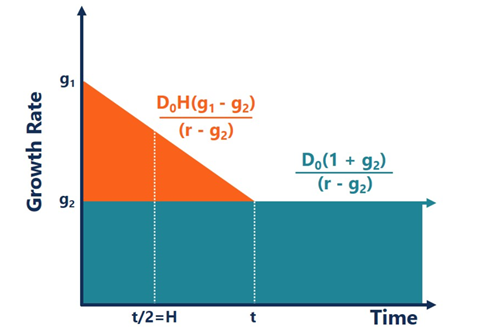
Terminal Value = (D0(1+g2))/(r-g2) + (D0*H*(g1-g2))/(r-g2)
D0 = Cash flow at terminal year
g1 = The initial high growth rate
g2 = The terminal growth rate
r = The discount rate
H = The half-life of the high growth period
However, due to difficulties of doing a normalization of cash flow with the H-Model, I would suggest you to extend the forecast period to consider the high growth period instead of using the H-model. In our example, we will stick to the Gordon Gorwth model as illustation.
The Exit Multiple Method
The exit multiple method is straight forward. You may view it as selling the business at the end of the forecast period based on an exit multiple. You may use all sort of market multiples such as P/E, P/S, P/B, EV/EBIT etc to compute an exit value and use it as the terminal value. We are not going to cover details of market multiples here, if you are interested, please go to here to learn more.
One common mistake made by people is that they simply add the terminal value derived directly to the present values of cash flows. Remember, the exit value computed is a value as of the terminal year, and we will need to convert it to present value by multiplying it with the terminal year’s discount factor.
When estimating the terminal growth rate, we usually benchmark it with the long-term GDP growth or inflation rate of the economy. Typically, perpetuity growth rates range between the historical inflation rate of 2 – 3% and the historical GDP growth rate of 4 – 5%. If the perpetuity growth rate exceeds 5%, it is basically assumed that the company’s expected growth will outpace the economy’s growth forever. There is a significant amount of judgement in the estimation of the terminal growth rate and determining when the company achieves steady-state and please make sure you are able to explain it with sound rationale when you decide to adopt certain number.
Some references include:
https://www.imf.org/external/datamapper/datasets/WEO the International Monetary Fund (IMF)
https://www.un.org/development/desa/dpad/resources.html?target=data United Nation’s Department of Economic and Social Affairs
From Enterprise Value to Equity Value
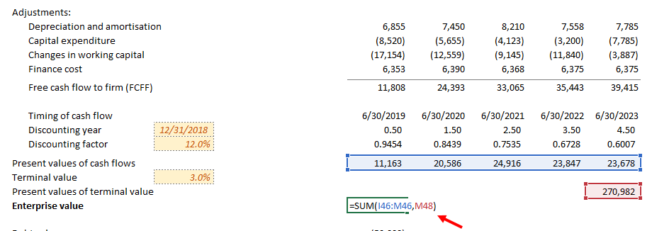
Now that we have the present values of both the projection period cash flows and the terminal value, we can compute the enterprise value by adding these present values together.
As mentioned earlier, enterprise value is the value of the business as a whole. To get the equity value, we need to deduct the debt value (because it belongs to the debt holder). You can get the debt value from the balance sheet of the business (sum of all borrowings) as of the valuation date. In our example, we assume the company has $50k debt.
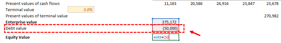
After deducting the debt value, you now have the equity value of the business (Finally!).
Marketability and Minority Discounts
Please note that the equity value here is on a controlling and marketable basis. You need to apply a discount if you are deriving the value of a private business or a minority stake of a business.
Marketability discount (DLOM)
You can sell shares in a listed stock at the click of a button, with a minimal brokerage cost; there is a visible level of investor demand. Selling shares in a private business is somewhat more laborious and more costly. There is no ready market, no button to click.
Take two identical businesses A and B. Company A is publically listed; company B is privately owned. Given the marketability advantage, a rational investor will prefer shares in company A over shares in company B. Consequently, assuming the market is efficient, an investor will be prepared to pay a higher price for shares in company A versus company B. In the DCF method, by default you will obtain a marketable equity value (because the market data you used in deriving discount rate are most likely from listed companies). To adjust it to reflect a value that
is non-marketable, a discount (DLOM) will need to be applied. Such discount could generally range from 5% to 50%. There are both qualitative and quantitative method to determine a DLOM which we will discuss further in future articles.
Minority discount / Discount on lack of control (DLOC)
A minority discount is the reduction applied to the valuation of a minority equity position in a company due to the absence of control. Minority shareholders usually have the inability to dictate the future strategic direction of the company, the election of directors, the nature, quantum and timing of their return on investment, or even the sale of their own shares. This absence of control reduces the value of the minority equity position against the total value of the company.
Let’s take a company that has two shareholders owning 70% and 30% each. If the company’s equity value is $10,000,000, a buyer looking to acquire the 30% position would not pay $3,000,000 because of the lack of control attached to this minority shareholding.
Similarly to the marketability issue, the result from DCF is on a controlling basis and you need a discount to convert it to a minority basis. Generally such discount would range from 10% to 30%, depending on various factors such as rights and protection to minority shareholders, nature of business etc. Unlike DLOM, DLOC is often determined with reference to these qualitative factors and it would involve significant degree of judgement.
If you need further help
When creative this step-by-step guide, we have tried to make it as clear as possible. But there are a lot more factors to consider in the real world and this guide alone may not be able to solve all the issues you could face in doing a DCF. If you need more help, you can always leave us comment or send us your questions, we will get back to you as soon as possible.
Alternatively, our team of valuation experts is also available to help you by providing a wide range of services. We charge a reasonable and transparent price and you can have a look at what we can offer here.